Research Highlights
This section is divided in three main areas:
2D Validation [S809 aerofoil]
NREL blade [Phase VI] (validation and the study of geometry variations).
Sliding-plane technique and some results that take into account the rotor/tower interaction or the rotor/wind tunnel walls influence.
LM19.1-like blade in the NTK-500/41-like wind turbine aerodynamic power analysis.
2D Validation [S809 aerofoil]
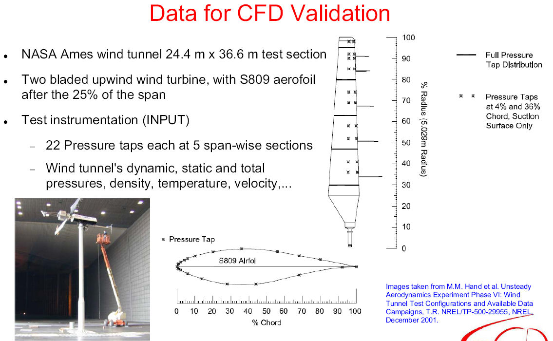
S809 aerofoil was selected for 2D validation due to its popularity, since it is referenced by several authors and also due to it was the aerofoil used in the NREL NASA-Ames Phase VI experiments that was a study case. The description of the aerofoil can be found clicking s809.dat and is shown in Figure 0.1.
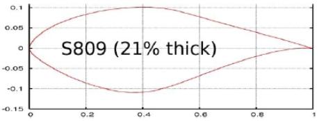
Figure 0.1
The grid used was based on the paper from Le Pape and Lecanu (Navier-Stokes Computations of a Stall-Regulated Wind Turbine, Wind Energy, 7(4):309-324,2004. DOI:10.1002/we.129) where 200 cells were distributed along the aerofoil, 57 cells at the wake and 61 cells normal to the aerofoil. Unsteady calculations were done above angle of attacks of 8 degrees obtaining solution every 1/50 degrees. The employed turbulence model was the k-w SST from Menter. The grid is shown in Figure 0.2:
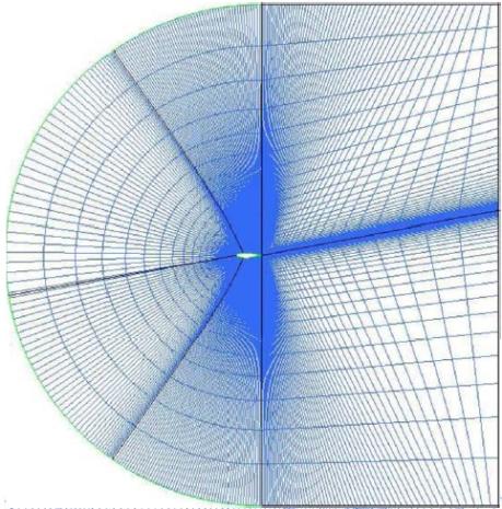
Figure 0.2
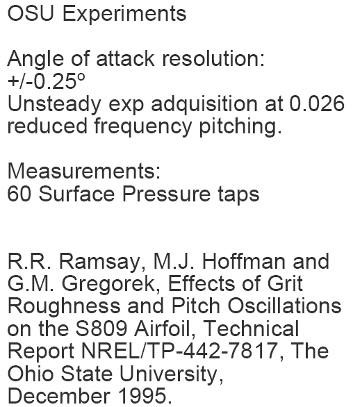
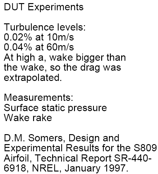
The lift, moment and drag coefficients along different angles of attack are shown in Figure 0.3 and the results obtained with WMB are compared with OSU (Ohio State University) (116kB) and DUT (Delft University) (106kB) wind tunnel experiments.
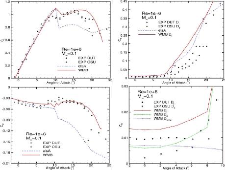
Figure 0.2
NREL Blade [Phase VI] (Validation and the study of geometry variations)
Results obtained using Liverpool CFD code (WMB) are presented.
For these calculations, isolated rotor was considered. The grid had 3,386,912 cells and 500 blocks in order to run it in parallel (for 24 CPU 98.7% balanced and for 48 CPU 97.2%). 174 cells were distributed chord-wise and 117 span-wise in each blade being the far-field located at 4 radii, inflow at 2 radii and outflow at 4radii.
The calculations are compared with the NREL Phase VI experimental data
(139kB) . In each figure the structured grid
(246kB) size and the turbulance model are given.
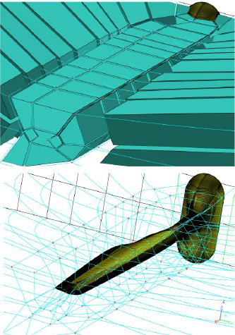
The geometries used for these cases are shown in Figure 1.1:
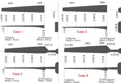
Figure 1.1
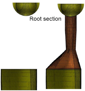
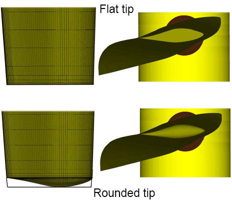
The main differences between these four geometries are in the root
(29kB) and tip
(40kB) sections. Case 1 & 2 are 5.4% longer than the experimental blade in order to analyze the influence of the tip vortex at the outboard stations and has not got any root attachment in order to quantify its importance when it is compared with experimental results and Cases 3 or 4. Case 3 & 4 have the same aspect ratio as the experimental blade and also a root attachment is modelled. The definition of the geometry for the experimental blades tip shape and root sections is not accurate enough to represent them exactly. Due to this Case 4 has a rounded tip having Cases 1-3 a flat tip. The root sections are modeled as a tube from inflow to outflow for Case 1, a spinner for Case 2 and the spinner with root attachment for Cases 3 & 4.
S070000 (7m/s 3deg pitch and 72rpm)
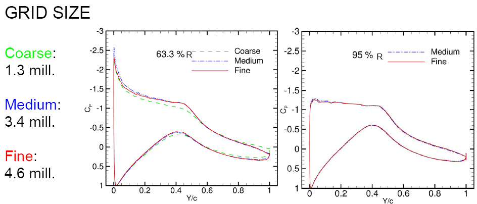
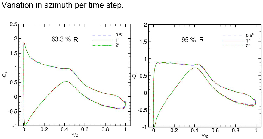
This case is the baseline case where the flow is attached and the agreements are good between the experiments and the CFD results. This case was also used for grid density validation
(165kB) , time step dependece
(164kB) analysis and to choose the location of the grid boundaries
(363kB)
3.3 million grid for the unsteady calculation with k-w turbulence model. Four spanwise sections are shown for all studied Cases: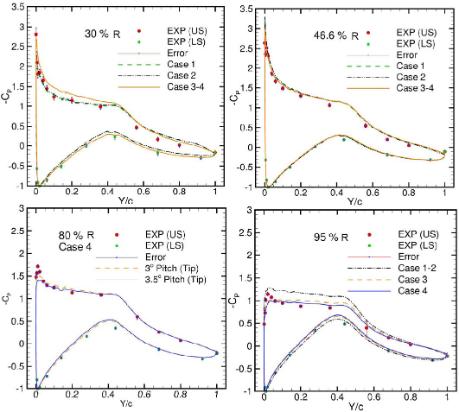
Figure 2.1
Experimental pressure coefficient and the tower influence are notable in the next figure. Due to that, sliding grid technique will be used to perform calculations where the tower influence or wind tunnel walls influences wants to be studied (see this poster for further details).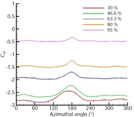
Figure 2.2
The wake at tip and root sections for the S070000 case with pressure as contour:
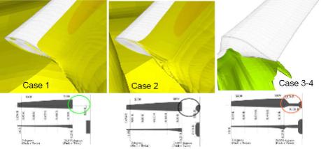
There is small root vortex variation between Cases 1 & 2. Case 3-4, in the other hand, has totally different vortex due to the root attachment, which reduces the strong vortex that can be appreciate in Cases 1 & 2.
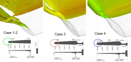
Figure 2.3
The tip vortex for Cases 1-3 develops closer to the leading edge than the Case 4 vortex, which is smoother and begins closer to the trailing edge due to its rounded geometry. The differences between Cases 1-2 & 3 are due to their different lenght. Cases 1-2 have larger lenght so the vortex is more separated to the tip end than Case 3.
The integrated loads for respect the azimuth and averaged one for all the Cases are shwon in the Figure 2.4:
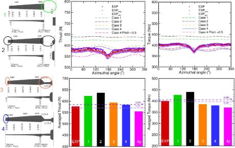
Figure 2.4
The local flow angles and the span-wise flow angles comparison is shown in Figure 2.5.
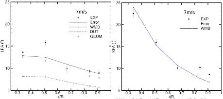
Figure 2.5
S100000 (10m/s 3deg pitch and 72rpm)
This situation is harder than the previous one due to the wind speed. This generates deattached flow in some parts of the wind turbine blades. This specific wind turbine was stall controlled (nowadays the majority of them are pitch controlled) so despite that in this case is also a desirable operational condition, this situation would try to avoid in contemporaneous wind turbines. Despite this, it is a very interesting case for studying due to the need of good turbulence and transitional modeling.
S100000 (10m/s 3deg pitch and 72rpm). 3.3 million grid for the unsteady calculation with k-w turbulence model (63.3% and 80% span station)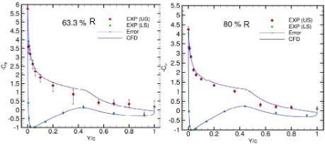
Figure 3.1
Averaged integrated loads for S200000 case are shown in Figure 3.2.
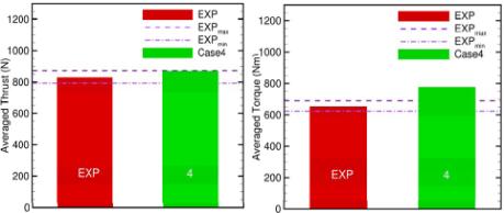
Figure 3.2
The local flow angles and the span-wise flow angles comparison is shown in Figure 3.3.
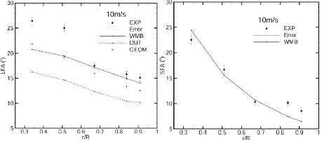
Figure 3.3
S200000 (20m/s 3deg pitch and 72rpm)
This situation is harder than the previous one due to the wind speed. This generates stall along the blades of the wind turbine. This specific wind turbine was stall controlled (nowadays the majority of them are pitch controlled) so despite that in this case is also a desirable operational condition, this situation would try to avoid in contemporaneous wind turbines. Despite this, it is a very interesting case for studying due to the need of good turbulence and transitional modeling.
S200000 (20m/s 3deg pitch and 72rpm). 6.5 million grid for the unsteady calculation with k-w turbulence model (63.3% and 80% span station)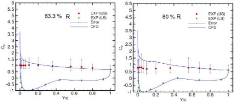
Figure 4.1
Averaged integrated loads for S200000 case are shown in Figure 4.2:
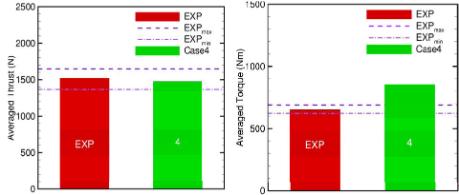
Figure 4.2
The local flow angles and the span-wise flow angles comparison is shown in Figure 4.3
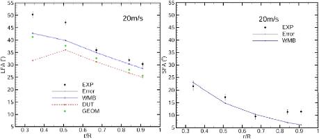
Figure 4.3
The wake for the S200000 case with pressure as a contour for unsteady computation is shown in Figure 4.4: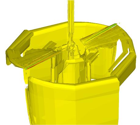
Figure 4.4
X070000 (7m/s 3deg pitch and 90rpm)
The 90rpm case is interesting due to the increase of the rotational speed. Nowadays, the wind turbine rotational speed is fix approximately at 300km/h tip speed, but the trend to do bigger wind turbines can be replaced with increasing the rotational speed taking into account the blade interaction effects.
X070000 (7m/s 3deg pitch and 90rpm). Steady computation at 1.4 million grid and k-w turbulence model. (63.3% span station)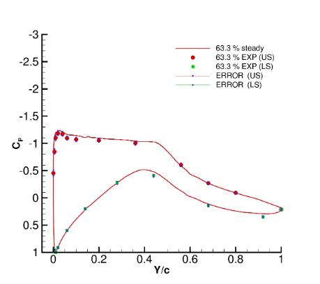
Figure 5.1
X070000 (7m/s 3deg pitch and 90rpm). 1.4 million grid for steady calculation with k-w turbulence model. Blade pressure along the span of the blade.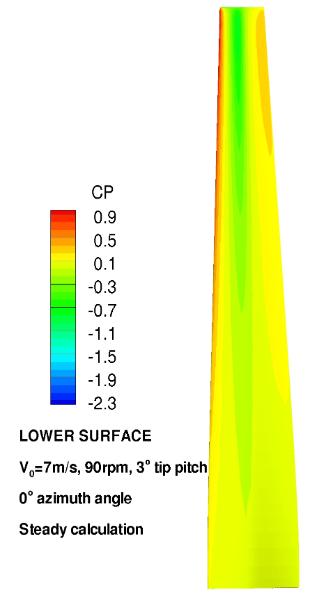
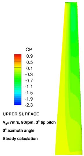
Figure 5.2
Sliding-plane technique and some results that take into account the rotor/tower interaction or the rotor/wind tunnel walls influence
A sliding-plane algorithm is used to account for the relative motion of the rotor and non-moving parts of the geometry, i.e. wind tunnel walls or the wind turbine tower and nacelle. An advantage of the sliding-plane approach over the more general overset-mesh or Chimera approach is that the computational overhead is limited due to the fact that the neighbour identifications and interpolations involve cells in two-dimensional plane, in contrast to the 3D overlaps resulting form employing the overset-mesh approach. For the cases considered here, the overhead added by the sliding-plane algorithm to the CPU time is typically around 4-5%.
The employed grid had ~7mill. cells and k-w turbulence model from Wilcox was used due to its robustness and it was computed for the S070000 (7m/s 3deg pitch and 72rpm) case. The sliding-plane location can be observed in Figure 6.1 as well as the blocking topology around the nacelle.
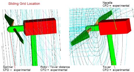
Figure 6.1
The torque calculations agrees well with the experiments and in Figure 6.2 the comparison between experiments and the WMB computations (with and without taking into account the tower) are shown.
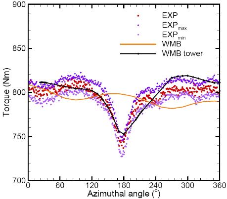
Figure 6.2
Pressure coefficient comparison show good agreement between the experiments and WMB results and 0/180 degrees azimuth positions are shown in Figure 6.3.
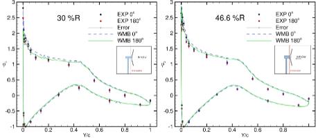
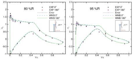
Figure 6.3
The interaction between the blade and the tower can be observed as well in the tower surface pressure variation (Figure 6.4).
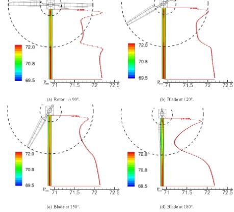
Figure 6.4
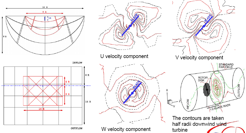
Finally, the iso-surface of Lambda 2 is coloured with distance from the wind turbine is shown in Figure 6.5 and a small video can be seen below.
