The Main Magnetic Field

The majority of the magnetic field we measure at the Earth's surface comes from sources internal to the Earth. By assuming that this field is a potential field, we can use the measurements of the magnetic field (especially from satellites) to construct a map of the large scale surface magnetic field (wavelengths greater than order 1000 km). In figure 1, we show such a model of the Earth's surface field, calculated using data from the CHAMP and Ørsted magnetic field satellites.

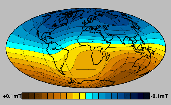
Radial magnetic field at Earth' surface

Unfortunately, the same potential theory that allows us to generate this map also tells us that formally we can say little more about the origin of the field. All we can say for sure is that it originates within the Earth, but where in the Earth cannot be distinguished. However, by looking at the structure of the field - and making assumptions about its sources - we are able to make further inferences. Figure 2 shows a spectrum of the field.

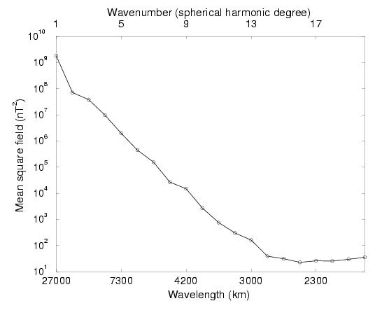
Spectrum of Field

We have plotted the mean square field at the Earth's surface as a function of the wavenumber of the field. It is clear that this spectrum has two parts, first a rapidly declining part down to wavelengths of approximately 3000 km, with a much more gentle decline at shorter wavelengths. We use the slope of the different sections in this spectrum to interpret the depth to the source of the field. The long-wavelength spectrum is consistent with a source at the core-mantle boundary (CMB), located at a depth of 2900 km. The CMB is the top of the accepted region of generation of the Earth's field - a hydromagnetic dynamo in the electrically conducting, liquid iron Earth's outer core. The spectrum at shorter wavelengths is consistent with much shallower sources, within the Earth's lithosphere - a combination of field induced by the core main field, and remnant magnetism from rocks that have cooled in the past, and have frozen in the ambient field at the time of their formation.

With these assumptions, we use the geomagnetic field to probe the structure and dynamics of the Earth. Figure 3 shows a map of the long-wavelength field in 2001 extrapolated to the CMB, on the assumption that the surface field with wavelength longer than 3000 km is dominated by this source (wavelenghts shorter than 3000 km arise from the lithospheric field).

Map of the long-wavelength radial field at the CMB

The Earth's continents are superimposed to provide a geographical reference. Compared with the map of the field at the Earth's surface (figure 1), the field is much stronger (compare the different scales), and the detailed field structure becomes clear; at the Earth's surface, shorter wavelengths are attenuated by distance from the source. The map we produce is similar to maps produced for previous times (in particular using data from the Magsat satellite from 1980, but also using historical data for earlier periods), but does show differences. In particular, the patches of magnetic field near the equator in the Atlantic hemisphere have been moving steadily westwards - it is this movement that produces the phenomena at the Earth's surface known as westward drift. However, this drift is far from uniform: in particular, strong concentrations of field at approximately ±70° latitude remain remarkably fixed over time.

We can use the change of the field with time (the secular variation) to elucidate the physics of the core. Imagine putting dye into a river. The movement of the dye will tell us about the structure of water flow in the river, until the dye eventually diffuses away. The magnetic field provides a similar tracer for the flow at the top of the core. From estimates of the electrical conductivity in the core, we believe that the effects of diffusion are small on time scales of less than a century: thus, we may use the secular variation to map the flow. While simple to state, this problem is not straight-forward: additional assumptions about the nature of the flow are required, in particular that it is large scale. Figure 4 shows a model of the flow at the surface of the core in 2001, calculated from a model of the magnetic field and secular variation determined from Ørsted data. Again, the continents are included only to provide a reference frame. Note the scale of the flow arrows: 20 km/yr is five orders of magnitude greater than the velocities of plate tectonic motion associated with flow in the Earth's mantle.

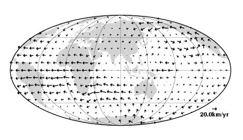
Flow at the surface of the Core at epoch 2001.0

We see several clear features, in particular a large counter-clockwise gyre under the Indian ocean, another under the Northern Pacific ocean, and strong westward flow under the Atlantic, which is responsible for the westward drift. Note however, that the equatorial flow under the Indian and Pacific oceans is much weaker, and in some places even eastward. This demonstrates clearly that to understand processes in the core, we must consider models of the magnetic field at the CMB, and not at the Earth's surface. Flow models such as produced here provide information about the dynamics of the flow in the core, allowing modelling of decadal variations in the rate of Earth rotation, and constraint of the computer simulations of the geodynamo that are being produced by a number of different groups. More details can be found in my article on Large Scale Flow in the Core, in the recently published Treatise on Geophysics.

Richard Holme (holme@liv.ac.uk)